Introducing Pivot Tables | Python Excels
A working knowledge of Microsoft Excel is now a prerequisite for just about every working professional using a computer on a regular basis. Excel training classes can be found in junior colleges, adult education centers, computer training centers, libraries, job search centers and of course online. Microsoft Excel basics is even taught in high schools.
But in my professional life, I've found few people who have a solid knowledge of pivot tables and are really comfortable using them in Excel. If you aren't aware of pivot tables or haven't had the time to try out this function in Excel, pivot tables provide a way to cross tabulate, sort, segregate and aggregate tabular data, enabling you to quickly summarize data and extract totals, averages, and other information from the source data. I first found out about pivot tables when I was working with our business unit financial analyst more than 10 years ago. She didn't like our corporate ERP system (SAP) any more than I did, and found it much faster to dump the raw data into Excel and get the answers to her questions by using a pivot table. I've been a pivot table convert ever since.
Using the spreadsheet newABCDCatering.xls developed in the last post, let's add a pivot table and answer the questions raised previously:
- What were the total sales in each of the last four quarters?
- What are the sales for each food item in each quarter?
- Who were the top 10 customers for ABCD Catering in 2009?
- Who was the highest producing sales rep for the year?
- What food item had the highest unit sales in Q4?
To build the pivot table, begin by selecting the entire data table in the Sheet2 worksheet by clicking cell A1, and typing the Control- key combination (hold down Ctrl and press ). This selects the data in the table without also grabbing blank cells surrounding the table. This is effectively the same as selecting cell A1 and scrolling to the last column and row of data while holding down the left mouse key.
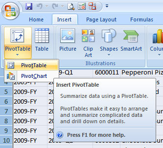
Next, if you're using Excel 2007 or later, select the Insert tab then select PivotTable from the Pivot Table icon
Because you've selected the spreadsheet data, the dialog should already be populated with the range Sheet2!$A1:$M791 as shown below
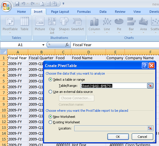
Click OK to create the empty pivot table.
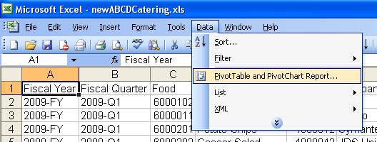
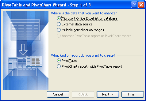
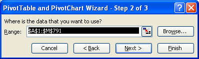
In Excel 2003 and earlier versions, select the table data as described above, then select Data->Pivot Table and Pivot Chart Report to create the pivot table.
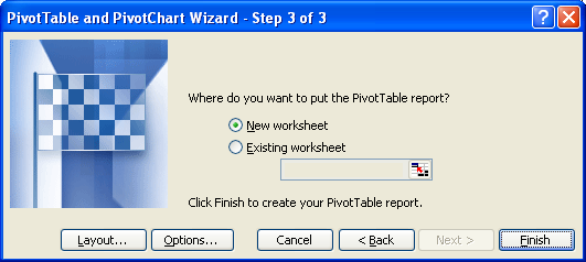
You're presented with a three step wizard. For now, just hit Next for the first two dialogs, thenFinish at the final dialog.
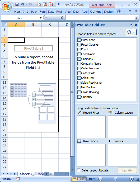
Once you've completed the above steps, you'll see the following displayed in older versions of Excel.
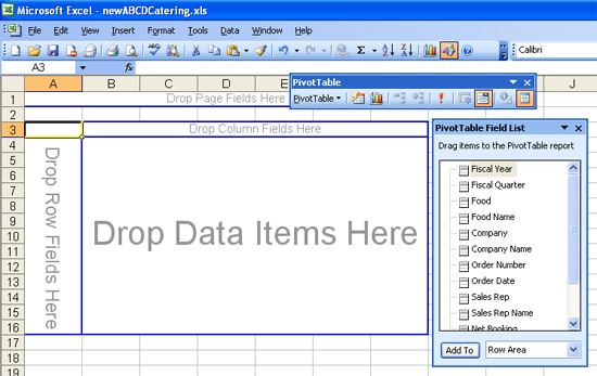
Now you're ready to do some data analysis.
What were the total sales in each of the last four quarters?
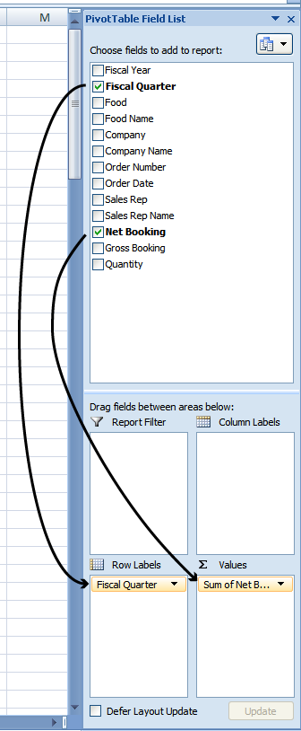
To understand the sales for the last four quarters, create a pivot table with "Fiscal Quarter" as a Row Label, and "Net Booking" as a Values field. To do this, drag the field "Fiscal Quarter" to the Row Labels section, and "Net Booking" to the Values section. (In older Excel versions, drag the "Fiscal Quarter" field directly onto the spreadsheet to the "Drop Row Fields Here" area, then drag the "Net Bookings" field onto the "Drop Data Items Here" area)
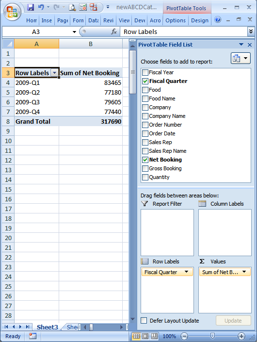
Your spreadsheet should now look something like this:
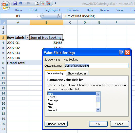
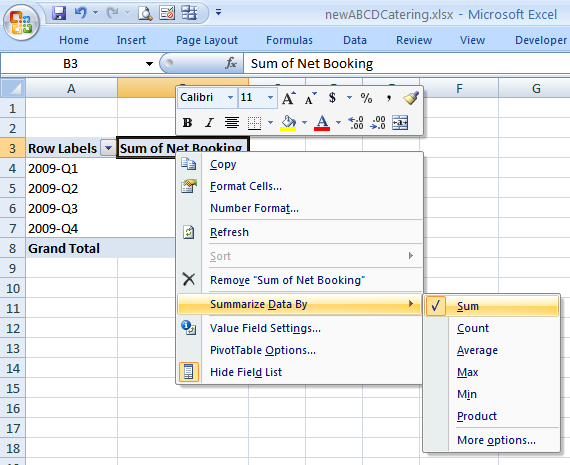
The header for the table data should say "Sum of Net Bookings". If it doesn't, double click on the header text and select "Sum" in the list box "Summarize value field by", or right mouse click over the text and select Summarize Data By->Sum.
Based on the spreadsheet data, the total net bookings in each of the last four quarters were $83465, $77180, $79605 and $77440 respectively.
What are the sales for each food item in each quarter?
To answer this question, we need the same fields as setup previously (Fiscal Quarter as a Row Label, Sum of Net Booking as a Value field), plus a column header for "Food Name". Remember that "Food" represents the numerical identifier for each food item, and "Food Name" contains the text description. Drag "Food Name" to the Column Labels section (in older versions of Excel, drag it to the "Drop Column Fields Here" area). The spreadsheet should now look like this:
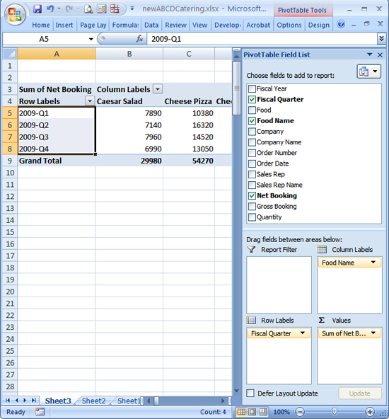
Note that each food item is listed as a column header, each of the four quarters are listed as row headers. Using this table you can quickly scan the data and understand the sales for each food item. For example, Caesar Salad sales were $7890, $7140, $7960 and $6990 in each of the respective quarters.
Who were the top 10 customers for ABCD Catering in 2009?
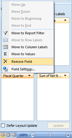
Again, Sum of Net Bookings is the data value, but we no longer need the Food Name or Fiscal Quarter data fields. Remove them by selecting them in the Row Labels or Column Labels boxes and dragging them back to the top, or by clicking the small triangle and selecting "Remove Field".
In Excel 2003 and earlier versions, select the column or row header and drag it back into the Field Chooser widget.
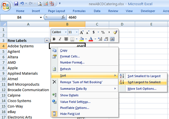
Now, add the Company Name field to the table by dragging it to the Row Labels box (or "Drop Row Fields Here" area in older Excel). The pivot table now contains the list of companies and their purchases, listed in alphabetical order. To find the top 10 customers, select the booking number for Adobe Systems, right click and select Sort->Sort Largest to Smallest
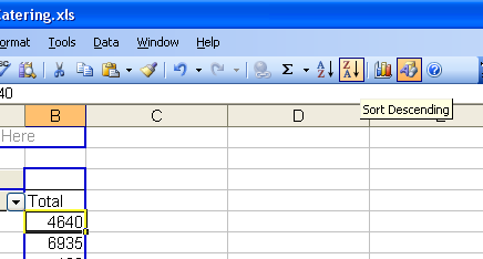
In older versions of Excel, select a booking number and click the "Sort Descending" icon in the tool bar, or select "Data->Sort" from the menu and select the descending sort.
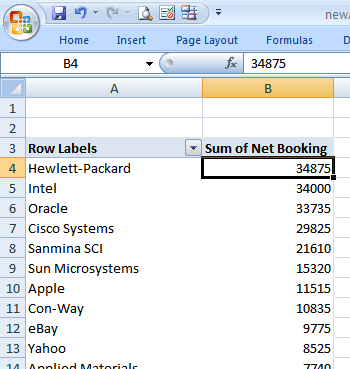
The list is now sorted, the top 10 customers for ABCD Catering are Hewlett-Packard, Intel, Oracle, Cisco Systems, Sanmina SCI, Sun Microsystems, Apple, Con-Way, eBay and Yahoo.
Who was the highest producing sales rep for the year?
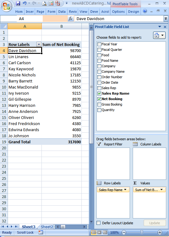
At ABCD Catering, sales reps cover multiple accounts. To find the highest producing rep, remove the Company Name field, replace it with the Sales Rep Name field and sort by Net Bookings. The top 10 sales reps are Dave Davidson, Lin Linares, Carl Carlson, Kay Kaywood and Nicole Nichols.
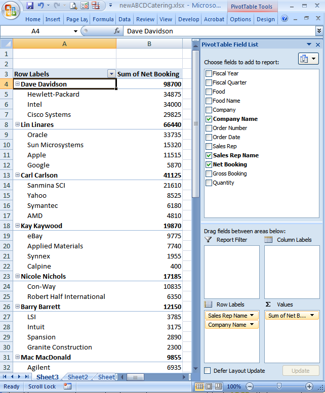
What accounts are these top reps responsible for? To find out, drag the Company Name field into the Row Labels area.
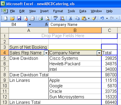
In older versions of Excel, drag Company Name directly onto the table
Since Hewlett-Packard, Intel and Cisco Systems were 3 of the top 4 producing accounts, it's no surprise that their sales rep Dave Davidson was the top performer.
Which food item had the highest unit sales in Q4?
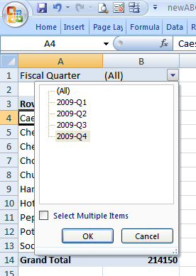
To find the food item with the highest unit sales, change the data value field to Sum of Quantity by removing Sum of Net Bookings, adding Quantity and making sure the Value Field Setting is "Sum" and not some other setting. Next, remove the Sales Rep Name and Company Name row header fields and replace them with Food Name. To limit the data to the Q4 quarter, drag the Fiscal Quarter field to the Report Filter area, and select "2009-Q4".
Finally, do a descending sort on the Sum of Quantity field to find the item with the highest unit sales.
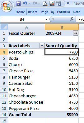
The number one item by unit volume was Potato Chips, followed by Soda and Churro.
Hopefully this gives you a feel for the power and flexibility of pivot tables. In the next post, we'll automate everything with Python and generate a simple framework for quickly building pivot tables.
Prerequisites
Microsoft Excel (refer to http://office.microsoft.com/excel)
Source Files and Scripts
The spreadsheet newABCDCatering.xls is available at http://github.com/pythonexcels/excelexamples/tree/master
Thanks — Dan