Mapping Excel VB Macros to Python Revisited
The last post introduced a technique for recording a Visual Basic macro within Excel and migrating it to Python. This exercise will build on those techniques while leveraging Python for more of the work.
This example creates two tables from scratch – a simple multiplication table and a table of random numbers – and applies conditional formatting to the numbers using some of the new features in Excel 2007 (unfortunately this exercise won't be compatible with older versions of Excel). Begin by starting the Python IDLE interface. Next, start Excel as you've done in the previous exercises. For this exercise, add a workbook using the Workbooks.Add() construct, and set the ws variable to point to the first worksheet in the workbook.
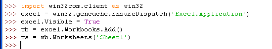
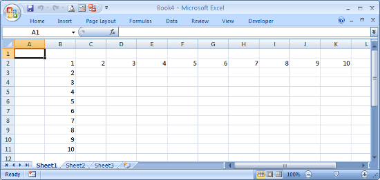
After typing these command in IDLE, you'll see the Excel window that contains an empty spreadsheet. To build the multiplication table, use Python to populate the column and row headers. There are a number of ways to do this, for this exercise you'll pass an list of column header and row header values to Excel. A row of data is defined by using the ws.Range().Valuestatement with a list or tuple on right hand side of the equals sign. Rather than explicitly defining the list as [1,2,3,4,5,6,7,8,9,10], you can use a functional programming statement containing a range() statement to populate the values: [i for i in range(1,11)]. The complete statement is ws.Range("B2:K2").Value = [i for i in range(1,11)]. Defining a single column of data is a bit trickier, you must define a list of single element lists or tuples. One way to do this is to use Python's zip() function to transpose the flat list into a list of tuples. The complete statement is ws.Range("B2:B11").Value = zip([i for i in range(1,11)]). The statements for completing the column and row headers are shown below.

At this point the column and row headers will appear in the Excel spreadsheet.
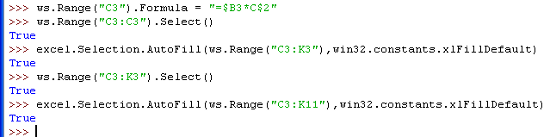
To define the product values for each cell in the table, create a formula to multiply the column and row header for a single cell, then used Excel to autofill the remaining cells. Looking at the spreadsheet, the product for cell C3 is cell B3 multiplied by cell C2, or 2 times 2 which equals 4. In terms of Excel, the formula is =B3*C2. To use Excel's autofill capability, you need to anchor the row and column in the formula by preceding it with the $ character. In other words, the formula you want to use is =$B3*C$2. Once that formula is entered, the expansion to fill the remaining cells is done in two steps. First, programmatically select the cell and drag it fill the row. Next, select the newly autofilled row and drag the new row down to fill in the remaining rows. Since this was demonstrated in the last post, please refer to that post if you need more information. The equivalent Python code to implement the autofill is shown below.
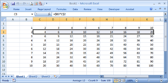
The spreadsheet will now contain the complete multiplication table.
To help illustrate conditional formatting, create another table of random integers between 1 and 100. Excel's RAND() function will generate a random number between 0 and 1, the formula we want is =INT(RAND()*100). The ws.Range().Formula construct can be used to fill a range with the same identical formula.
The Excel spreadsheet should now contain both the multiplication and random number tables.
Now that the data is ready, conditional formatting can be applied. Even though you invoked Excel from Python, you still can manipulate the spreadsheet using the Excel interface, and even record macros. You need to record a macro like you did in the last post in order to capture the VB commands, so click on Record Macro in the Developer tab, then click OK in the popup dialog.
Select all the cells in the range B2:K22. In the Home tab, select Conditional Formatting->Color Scales->Red-Yellow-Blue Color Scale.
The spreadsheet should now show a color background for each of the selected cells containing a value. Now select cell A1, then stop the macro by clicking Stop Recording in the Developer tab.
Your spreadsheet will now have conditional formatting applied and will look something like this, with cells containing numbers near 100 colored in Red, cells with a value of 50 in Yellow, and cells with a value of 1 in Blue, with a shade of these colors for values in between:
As an aside, you can update the random numbers in the lower table by hitting the F9 key to force a spreadsheet recalculation.
To continue, open the macro just created by selecting Macros from the Developer tab, select the name of the macro you just captured and click Edit. The macro should look something like this:
Sub Macro1()
'
' Macro1 Macro
'
    Range("B2:K22").Select
    Selection.FormatConditions.AddColorScale ColorScaleType:=3
    Selection.FormatConditions(Selection.FormatConditions.Count).SetFirstPriority
    Selection.FormatConditions(1).ColorScaleCriteria(1).Type = _
        xlConditionValueLowestValue
    With Selection.FormatConditions(1).ColorScaleCriteria(1).FormatColor
        .Color = 13011546
        .TintAndShade = 0
    End With
    Selection.FormatConditions(1).ColorScaleCriteria(2).Type = _
        xlConditionValuePercentile
    Selection.FormatConditions(1).ColorScaleCriteria(2).Value = 50
    With Selection.FormatConditions(1).ColorScaleCriteria(2).FormatColor
        .Color = 8711167
        .TintAndShade = 0
    End With
    Selection.FormatConditions(1).ColorScaleCriteria(3).Type = _
        xlConditionValueHighestValue
    With Selection.FormatConditions(1).ColorScaleCriteria(3).FormatColor
        .Color = 7039480
        .TintAndShade = 0
    End With
    Range("A1").Select
End Sub
Though the macro contains some very long method names, plus some With statements, the porting will be very straightforward. Here are some guidelines to keep in mind while migrating this code to Python.
Selectionis preceded byexcel.
Remember that Selection is a method at the Excel Application level, you need to precede it with excel. in this example.
Rangeis preceded byws.
Range is a method at the Worksheet level, which is defined earlier as ws. in this example.
- Function calls require
()in Python
Unlike VB, any function calls must by followed by () in Python.
Withstatements must be expanded
The three With blocks in this macro need to be expanded, which can be done with temporary variables or by copying the statement following the With keyword. For example, the first Withblock:
With Selection.FormatConditions(1).ColorScaleCriteria(1).FormatColor
    .Color = 13011546
    .TintAndShade = 0
End With
can be written in Python as
excel.Selection.FormatConditions(1).ColorScaleCriteria(1).FormatColor.Color = 13011546
excel.Selection.FormatConditions(1).ColorScaleCriteria(1).FormatColor.TintAndShade = 0
or by using a temporary variable as
x = excel.Selection.FormatConditions(1).ColorScaleCriteria(1).FormatColor
x.Color = 13011546
x.FormatColor.TintAndShade = 0
Temporary variables were created to make the script more concise. In particular, the statement [csc1,csc2,csc3] = [excel.Selection.FormatConditions(1).ColorScaleCriteria(n) for n in range(1,4)] was used to create three temporary variables for the three ColorScaleCriteria methods. The equivalent Python text representing the macro is shown here:
To save the spreadsheet and close Excel, use the SaveAs and Quit methods as shown below.
Here is the
complete conditionalformatting.py script. The line excel.Visible = True has been commented out. Unless you are developing the script, you typically want Excel to run invisibly in the background.
#
# conditionalformatting.py
# Create two tables and apply Conditional Formatting
#
import win32com.client as win32
excel = win32.gencache.EnsureDispatch('Excel.Application')
#excel.Visible = True
wb = excel.Workbooks.Add()
ws = wb.Worksheets('Sheet1')
ws.Range("B2:K2").Value = [i for i in range(1,11)]
ws.Range("B2:B11").Value = zip([i for i in range(1,11)])
ws.Range("C3").Formula = "=$B3*C$2"
ws.Range("C3:C3").Select()
excel.Selection.AutoFill(ws.Range("C3:K3"),win32.constants.xlFillDefault)
ws.Range("C3:K3").Select()
excel.Selection.AutoFill(ws.Range("C3:K11"),win32.constants.xlFillDefault)
ws.Range("B13:K22").Formula = "=INT(RAND()*100)"
ws.Range("B2:K22").Select()
excel.Selection.FormatConditions.AddColorScale(ColorScaleType = 3)
excel.Selection.FormatConditions(excel.Selection.FormatConditions.Count).SetFirstPriority()
[csc1,csc2,csc3] = [excel.Selection.FormatConditions(1).ColorScaleCriteria(n) for n in range(1,4)]
csc1.Type = win32.constants.xlConditionValueLowestValue
csc1.FormatColor.Color = 13011546
csc1.FormatColor.TintAndShade = 0
csc2.Type = win32.constants.xlConditionValuePercentile
csc2.Value = 50
csc2.FormatColor.Color = 8711167
csc2.FormatColor.TintAndShade = 0
csc3.Type = win32.constants.xlConditionValueHighestValue
csc3.FormatColor.Color = 7039480
csc3.FormatColor.TintAndShade = 0
ws.Range("A1").Select()
wb.SaveAs('ConditionalFormatting.xlsx')
excel.Application.Quit()
Prerequisites
Python (refer to http://www.python.org)
Win32 Python module (refer to http://sourceforge.net/projects/pywin32)
Microsoft Excel (refer to http://office.microsoft.com/excel)
Source Files and Scripts
Source for the program conditionalformatting.py script is available at http://github.com/pythonexcels/examples
That's all for now, thanks — Dan